Sunday, October 26, 2014

Post #3. Sinusoidal functions and Sinusoidal gratings

One issue of my interest have been to programm visual stimuli in order to use in vision research. Classically, a very useful stimulation for visual system investigations is named sinusoidal grating. The sinusoidal gratings are the graphical representation of the luminance or color modulation following a sinusoidal function. Here, I'll show how to program sinusoidal functions and its correspondent sinusoidal grating.
First, let's create sinusoidal function with the code below. It is important to set the free parameters of the sinusoidal functions: frequency, amplitude, and phase.

frequency = 1;%Set the frequency
phase = 90;%Set the phase in degrees that needs to be converted to radians
amplitude = 1;%Set the amplitude
x = 0:0.001:1;%x domain 
wave = amplitude*sin((2*pi*frequency*x)+(deg2rad(phase)));
plot(x,wave,'k','Linewidth',2)
axis square 
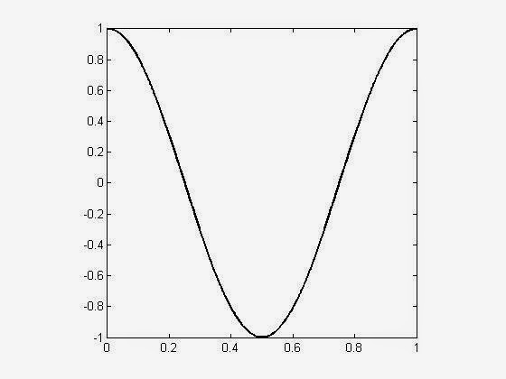
Fig 01. Graphical representation of the sinusoidal function set in the code above (frequency = 1; phase = 90 deg; amplitude = 1). 

Now, I'll show how to use the sinusoidal function to modulate the spatial luminance to create sinusoidal gratings. The code below use introduces the functions meshigrid( ) and surf( ). The function meshgrid( ) are used to create a square matrix that will be used to be modulated by the third dimension, the spatial luminance. The surf( ) function is used to make three dimensional shaded surface plot.

%We set the same previous parameters
frequency = 1;
phase = 90;
amplitude = 1;
[X,Y]=meshgrid(0:0.001:1,0:0.001:1);
Z = amplitude*sin((2*3.1415*frequency.*X)+(phase));
surf(X,Y,Z)
shading interp
view(0,90)
colormap gray
axis off
axis square
Fig 02. Luminance spatial sinusoidal grating for the parameters of the code above (frequency = 1; phase = 90 deg; amplitude = 1). Look the luminance is following the profile of the plot in the Figure 01.

Now, try to change the parameters to visualize other several sinusoidal waveforms. Below, more examples of sinusoidal functions and its correspondent sinusoidal grating. To know better about meshgrid( ) and surf( ) functions read the MATLAB help. 


frequency = 4, phase = 0; amplitude = 1               frequency = 10, phase = 270; amplitude = 1 


Any doubt, contact me in givagosouza@gmail.com

Saturday, October 18, 2014

Post #2. Choosing the file address to import datafiles

Someone, who works with stored data and needs to import new datafiles from different folders every time, needs to know how to import datafiles from specific folder address. In MATLAB, there is a function that help us with the task to looking for the desired folder. The function is uigetfile( ). This function opens the standard dialog for retrieving files. Specially for begginners, I'll indicate a code that introduces the use of this function.
The code starts with:

[file,dir] = uigetfile('.txt','Select file to import');


This line will make appear a open standard dialog box as showed below in the Fig 01.

Fig 01. Open standard dialog box. The title of the dialog box ('Select file to import') and the type of file ('.txt') to be imported were set in the command line above.

Once you chose the file to be imported, the function returns the value to the variables [file,dir]. The variable file will save the file name, and the variable dir will save the folder address. In the previous example, the variable file will be 'example.txt' , and the variable dir will be 'C:\Users\hp\Desktop\ '. Both information together will constitute the complete address of the file. The next line will concatenate the variables dir and file. 

FileToOpen =  [dir file];

The line above concatenated the both variables with [dir file], and the variable FileToOpen will receive the complete address of the file ('C:\Users\hp\Desktop\example.txt' ) to be imported.

The next lines will be used to evaluate if the variable FileToOpen is not valid. If it is ok, a new variable named Data will receive the information of the import command importdata( ) of the file addressed in FileToOpen. Finally the stored data will be ploted.

if FileToOpen ~= 0
    Data = importdata(FileToOpen);
    plot(Data(:,1),Data(:,2),'o')
else
end

This simple code can also be used to import different datafiles such as .csv and .mat. Any doubt contact me in givagosouza@gmail.com


Sunday, October 12, 2014

Post #1. High quality plot in MATLAB

It's my first post in this blog. My purpose is to open a link of communication with other people that wants to get more experience in the use of MATLAB programming for technical and scientific reasons or even just for fun. My first issue to discuss is how ugly or pretty can be the plots created in MATLAB. During the last seven years, I always thought that it would be impossible or I would spent lot of energy to make pretty plots using MATLAB. I used to process the data in MATLAB. After that, I exported the processed results to text file, and finally, I made the plots in Microsoft Excel. Obviously, I was doing something wrong! 
Today I'm posting a code to customize plots in MATLAB in order to make them more beautiful.
Look the plot below. This is one example of ugly plot made by using the default properties of MATLAB.

 Fig 01. An example of plot made using the default plot properties of MATLAB. Ugly plot!

The plot in the Fig 01 was created using the following simple code:

x = 1:10;       %Data from x domain
y = x+2;        %Data from y domain
plot(x,y,'o');  %Function to plot the data
axis square   %Command to make squared plots 
xlabel('X')    %Command to name the x domain
ylabel('Y')    %Command to name the y domain

Look now the same data with some changes in plot properties.
Fig 02. An example of a plot with the same data in the Fig 01, but with changes in many plot properties.

The Fig 02 was made using the still simple code:

x = 1:10; %Data from x domain
y = x+2; %Data from y domain

plot(x,y,'o','MarkerEdgeColor',[0.1 0.1 0.1],'MarkerFaceColor',[0.8 0.8 0.8],'MarkerSize',12); %Function to plot the data. Here, I change plot properties of the color of the maker edge and marker %face and the marker size.

axis square

%Two lines below, I set the font name, font size, and the font weight. I did using my preferences. 
xlabel('X','FontName','Times New Roman','Fontsize',18,'Fontweight','bold')
ylabel('Y','FontName','Times New Roman','Fontsize',18,'Fontweight','bold')

%Below, I changed many plot properties that in my opinion give more visibility to the graph
set(gca,'Box', 'off', 'TickDir', 'out', 'TickLength'  , [.035 .035] , 'XMinorTick'  , 'on', ...
'YMinorTick', 'on', 'YGrid', 'on', 'XGrid', 'on', 'LineWidth', 3, 'FontName', 'Times New Roman',...
'Fontsize',18,  'Fontweight','bold');

After you write the code to customize the plot, it is necessary only to apply the same code for new plots. I know that the beauty is in the eye of the beholder, and it doesn't matter if the Fig 02 is prettier than Fig 01, but with few more lines in your code you can change the quality of your data presentation.

Feel free to contact me about this post or other MATLAB issues by the e-mail givagosouza@gmail.com